Maximize your fluorescence imaging throughput with the Nucleus Microscopy Platform
By Mike Fussell, Marketing Team
Published on May 26, 2022
Compared to conventional manual microscopy, automated microscopy delivers high quality data by improving consistency and eliminating the chances of missed steps in imaging protocols. Automation also enables the rapid acquisition of data from large areas or many microplate wells. Optimizing the performance of automated microscope systems to maximize imaging throughput can improve your productivity, saving you time and money. The Nucleus® automated microscopy platform provides a complete set of interchangeable hardware modules and software tools for building your bespoke inverted or upright standalone microscope or optical subsystem.
Contributors to Throughput
The overall throughput of your microplate and slide scanning system will depend on the combined times for each step of your image acquisition process. While some steps like the movements between imaging positions and exposure times are more obvious, there are several other steps including device communication, and system latency that are frequently overlooked. These additional steps can have a big impact on your overall throughput.
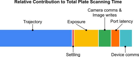
Figure 1. Each step of the sample positioning and image acquisition process contributes the total time required to scan a single 96-well plate with a 25ms exposure at each well. The relative impact of each step will depend on the number of wells to be imaged, how many images are captured per well and the exposure duration for each image.
Identifying the relative contribution of each step in your imaging process will help identify the steps which can be optimized that will have the largest impact on your throughput. This will help to focus your attention where it can deliver the biggest improvements first. For example, when imaging bioluminescent samples with 20 minute exposure times on a 6-well plate, saving a 1 second per well will not yield a significant improvement in throughput. However, the same time saving when imaging three fluorophores on a 1536-well plate with a short exposure time will save more than 76 minutes per plate, yielding a significant boost in throughput.
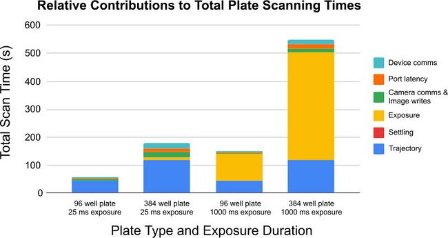
Figure 2. As exposure times and well counts change, the relative contribution of each step in the image acquisition process to the overall plate scanning time changes. With short exposures, optimizing the movement profile to decrease movement and settling time will yield the biggest improvement in throughput. As exposure times increase, they quickly become the largest contribution to overall scanning time.
Movement
Speed and Acceleration
At first glance, choosing a stage with the fastest possible maximum speed may seem like the most obvious way to increase your throughput. While this may be true for many motion control applications, for microscopy raw speed alone is of limited benefit and in some cases may actually reduce your throughput. For the small, repeated movements which are typical of scanning microplates or slides, acceleration is more important than maximum speed as the movements between wells are so short that there is insufficient distance for the stage to reach its maximum speed.
| Stage Series | Stage Drive | Max. Speed. | Min. 96 Well Scanning Time | Min. 384 Well Scanning Time |
|---|---|---|---|---|
| X-ADR | Linear Motor | 750 mm/s | < 12 Seconds | < 46 Seconds |
| X-ASR | Stepper Motor | 85 mm/s | < 19 Seconds | < 58 Seconds |
Table 1. The minimum scanning time is the time required to traverse a standard microplate with a 100X objective stopping at each well to settle and capture a 25 μs exposure. Scanning times will vary on a case-by-case basis depending on camera, fluorophore, imaging parameters, illumination wavelength and objective selection. Stage service life will vary depending on the stage load, speed and acceleration. Higher loads at higher speeds will result in increased wear of stepper motor stage components.
This effect explains the difference between the scan times of a 96 well and 384 well microplate when imaged with a high-speed linear motor-driven X-ADR stage vs a stepper motor-driven X-ASR stage (Table 1). At their maximum speed, X-ADR stages are 8.8 times faster than X-ASR series stages, however, over the short distances between microplate wells, they don’t have time to reach that maximum speed. The higher maximum acceleration of X-ADR stages when positioning a typical load like a 96-well plate will deliver an improvement in throughput. However, as plate density increases, the shorter well-to-well distances (Fig. 3) reduce the time the stage has to get up to full speed. This results in a smaller difference between linear motor and stepper motor stages on higher density plates.

Figure 3. Over short distances (1, 2), neither stage can reach its maximum speed and acceleration will have a greater impact on overall scanning time. As movement distances increase further (3), the benefit to scanning time of X-ADR stages’ high acceleration also increases
Accuracy and Repeatability
A high maximum movement speed and acceleration are not enough to guarantee an increase in throughput. Rapid movements are of limited value if a stage does not arrive at the target position and further fine position adjustment steps are required. Two key properties of a microscope’s motion control systems are accuracy and repeatability.
Accuracy
Accuracy is the maximum error possible when moving between any two positions on a stage, when both positions are approached from the same direction. A stage with greater accuracy will deliver increased throughput by eliminating the need for fine-repositioning to reach a target position. With a high-accuracy stage, the overlap required to ensure complete coverage of a stitched XY area scan can be minimized, reducing the total number of images required.
The reported accuracy spec of stepper motor-driven stages is the maximum possible error when moving between two points on a stage. Accuracy of stepper motor stages is inversely proportional to the length of their travel as the influence of small variations in their lead screw drives accumulate over their length. Over short distances the accuracy of stepper motor stages is typically much higher than the “worst case scenario” reported in the spec. Linear motor-driven stages maintain a constant accuracy across their entire range of travel.
Repeatability
Repeatability is the ability of a stage to return to the same position from the same direction multiple times. High repeatability of a focus stage enables highly consistent Z-stacking. This can yield greatly improved throughput for multi-channel Z-stacked imaging by enabling an optimized scanning sequence which minimizes filter cube switching. This will be explained in greater detail below. The repeatability of both stepper motor and linear motor-driven stages is independent of the length of their travel.
Settling Time
Once the sample has been moved to the correct position for image acquisition, it must come to a complete stop before a clear image can be acquired. Settling time is the time required for any vibrations resulting from the movement of the stage to dissipate enough to capture a sharp image. For most applications this means the movement in the sample will be less than a 1 pixel.
X-ADR linear motor-driven stages achieve their < 0.5 µm repeatability specification with the help of a 1nm resolution optical encoder. By directly measuring the stage position, the X-ADR’s integrated controller can approach the target position and automatically compensate for overshoot. The fine resolution of X-ADR series stages’ encoders allows them to make increasingly fine adjustments to the stage position to approach the target position as closely as possible. To maximize your imaging throughput, use the cloop.settle.tolerance setting to adjust the settling threshold to the largest value which still produces acceptably sharp images under your imaging conditions.

Figure 4. Exposure A is acquired immediately after a movement before the stage has settled resulting in a blurry image. By allowing time following the movement for the stage to settle, exposure B delivers a clear image.
For movements over very short distances, the settling time can be longer than the movement time. It can seem counterintuitive, but for short distances, reducing the speed and acceleration can often improve throughput by reducing the settling time. Reducing the maximum speed and applying an S-curve motion profile helps prevent jerking motions which require longer settling times. Increasing the motion.accel.ramptime setting will result in a smoother more pronounced S-curve motion profile which will settle more quickly. Securely mounting your microscope to an optical table can greatly reduce the settling time, enabling more images to be captured in less time.
The appropriate settling time will depend on the magnification of your objective, and the requirements of your application. Imaging for research applications where differentiating between fine structures is crucial may require much clearer images than reading an assay where simply detecting a fluorescent signal is adequate.
Zaber microscope stages use crossed roller bearings in the LDA focus stage, and ADR and ASR XY stages to achieve very high stiffness and short setting times. Zaber ADR stages with 1nm resolution optical encoders can directly measure stage vibrations and trigger image acquisition once a target threshold has been reached using the cloop.settle.tolerance setting. This can increase throughput by triggering as soon as possible, rather than waiting for an arbitrary settling period.
Input shaping & Trajectory optimization
Optimizing the motion profile of a stage can deliver very significant improvements in throughput. Excluding camera and illumination settings which can shorten the total image acquisition time, trajectory optimization can provide the biggest improvement in throughput (Fig. 5).
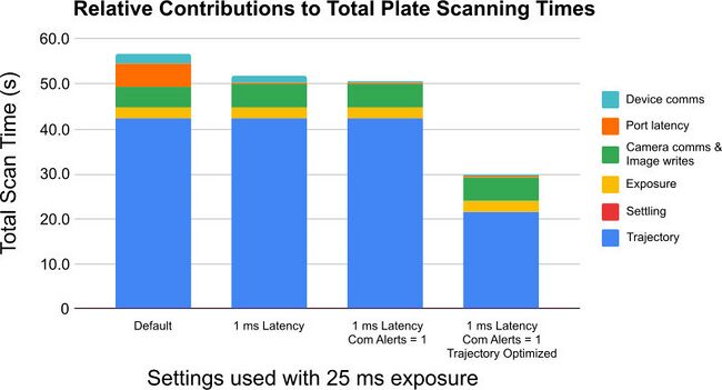
Figure 5. Impact of on scanning time of a 96-well plate of reducing the Windows serial port latency timer to 1 ms, enabling comm.alert, and updating the setting motion.accelonly = 1000, motion.decelonly = 1200, maxspeed = 630000 and motion.accel.ramptime = 5 to produce a more aggressive motion profile without incurring an increased settling time penalty.
A very aggressive motion profile with a high acceleration may overshoot (Fig. 5) the target position and a correction which will add additional time to the final move. A smoother, slower movement which arrives directly at its target position may take longer to initially reach that position, but will not require additional position correction.
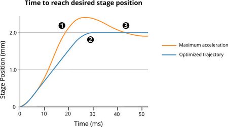
Figure 6. Maximum acceleration on an X-ADR stage will result in the stage reaching the target position quickly (1) but overshooting it and requiring further position adjustment to approach the target position (3). An optimized motion profile will be slower to reach the target position, but will not require additional adjustment.
The Oscilloscope tool in Zaber Launcher software can record the position information from the optical encoder in X-ADR stages. This data takes the guesswork out of optimizing movement profiles and makes evaluating the impact of changes in speed, acceleration, and acceleration ramp time easy.
Scanning Sequence Optimization
Optimizing your scanning sequence to minimize unnecessary movement and image acquisition steps can yield a significant reduction in overall scanning time. As microplate density is increased and additional imaging dimensions are added, sequence optimization becomes increasingly critical as even small improvements can save many minutes when multiplied out across many wells, illumination channels and z-stack layers.
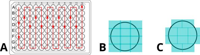
Figure 7. Plate-level and well-level scanning patterns should both be optimized. Optimizing the well to well scanning path saves time by minimizing the movement. Optimizing the number of images per well and their positions (A, B) can have very significant impacts on overall scanning time. The benefits of such optimization increase as more Z layers and fluorophores are added to the imaging protocol.
When planning a sequence of many short movements on an XY state, orienting those movements along the upper axis of the stage is preferable. The upper axis which is only moving its own mass, plus the sample will move and settle faster than the lower axis which must move its mass, plus the mass of the sample and the upper axis.
Multi-Dimensional Imaging
Many research and commercial imaging applications require data at more than one excitation wavelength, focus position and point in time. Each of these dimensions adds additional complexity to the image acquisition process. As multiple dimensions are combined, the value of optimizing your scanning pattern increases dramatically. To acquire data from a single XY position at 3 focal planes using 3 excitation wavelengths over three points in time requires 27 images. This translates into 2,592 images for a full 96-well plate (Fig. 8).
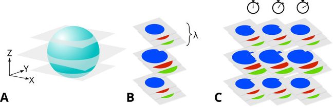
Figure 8. 3D imaging (A) results in a stack of images with the focal plane at different depths. 4D imaging (B) captures a stack of images at multiple depths and with multiple emission/excitation filters. Increasing the depth of magnitude of dimension will result in a significant increase in overall capture time. 5D imaging (C) captures time-resolved sequences of images.
The rapid expansion in the number of images required when combining multiple dimensions to your image necessitates careful planning of your imaging sequence to eliminate unnecessary steps, and organize essential steps in the most efficient way.
Consider the sequence of 9 images required for a 3-plane Z stack at three excitation wavelengths (Fig. 9). At 350 ms, the filter cube switching time of a Nucleus® microscope is significantly longer than the movement and settling time of its X-LDA focus stage. By reducing the total number of filter cube changes, scanning each layer of the Z-stack at one wavelength, then switching the filter cube and re-scanning the Z-stack at the new wavelength is much faster than imaging each layer with all three wavelengths then moving to the next layer of the stack.
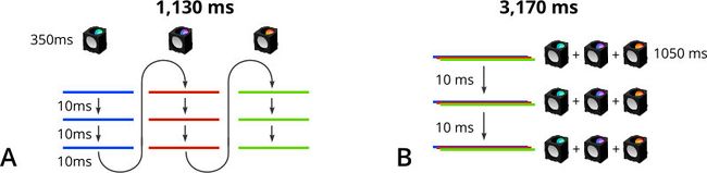
Figure 9. Two multi-channel image acquisition sequences compared. Imaging each layer of the Z stack, then changing filter cubes (A) is much faster than imaging a single layer with all three channels before moving to the next layer (B). This example ignores image exposure times which would be the same for both cases.
Translating this example to a 96-well plate, this scan optimization would save 3:15 per plate. The relative impact this will have on overall throughput will depend on image acquisition time which will be the same for both cases.
This method of sequence optimization relies on having a focus stage with a high repeatability. Repeatability is critical to ensuring that the images from one wavelength Z stack will be captured at the same focal plane as subsequent Z-stacks. To maximize the repeatability of the focus stage positioning, approaching the target focus point from the same direction each time is preferable.
Focus Interpolation
At high magnifications, the typical variability in microplate flatness may cause a shift in the ideal focus distance across the surface of the plate. Most microscope control software packages have image-based autofocus methods which can be called to determine the optimum focus. These methods capture a stack of images of different focal distances and compare them to determine the ideal focus position. While accurate, image-based autofocus at every well would greatly increase the time required to image a plate.
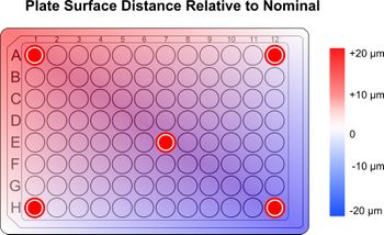
Figure 10. Focus points selected for interpolation.
By determining the ideal focus at each corner and the middle position, and interpolating between these points for the intermediate wells can deliver more accurate results while being 19 times faster than performing autofocus on every well. The Scipy Python library provides a cubic interpolation function which is useful for creating a smooth curve between adjacent focus positions.
This approach will work with adherent cells located on the bottom of each well. This approach may not perform as well on general purpose plates, which may see a variance in bottom height of wells spaced one apart by up to 20 μm. Higher quality plates intended for imaging use and manufactured to tighter tolerances will maintain a more consistent focus across the plate reducing the need to refocus.
Image Acquisition
To achieve the fastest imaging performance, the Illuminator, filter set, fluorophore, and camera must all work together. To achieve the optimum throughput, the illuminator must excite the fluorophore with enough intensity to achieve the desired signal to noise ratio (SNR) of the experiment with as short an exposure as possible.
Illumination
For most applications, increasing the intensity of illumination will enable shorter exposure times and increased throughput. Some fluorescence applications may require extremely high intensity excitation illumination or illumination at wavelengths outside the standard MLRA and MLRB epi illuminators. To support these use-cases, Nucleus microscopes are compatible with 3rd party illuminators using a common 3mm liquid light guide. For many biological imaging applications, photobleaching of fluorophores and phototoxicity to live cells will impose an upper limit on the maximum intensity of light the target can safely be exposed to.
When imaging multiple fluorophores using a single multiband filter set to eliminate filter cube switching, the LED channel switching speed should be considered. To avoid two fluorophores being excited simultaneously, LED channels must be completely switched off. The faster an LED controller can completely switch off one channel and switch the next channel on, the higher the system’s throughput will be.
The emission spectra of the illuminator must also be considered when selecting complementary fluorophores and filter sets. The Semrock Searchlight tool which includes data from the Nucleus MLR3A and MLR3B illuminators is a useful tool which can aid with filter set selection.
Camera Selection
When adding more light through illumination is not practical, a camera with greater sensitivity is the next best option to reduce exposure times. The camera used to acquire images of a sample can have a major impact on the overall throughput of an automated microscope. The resolution, readout architecture and interface determine the maximum speed the camera can operate at.
Selecting a camera with a high-speed interface is crucial to achieving a high throughput with your microscope. The interface will determine the number of pixels per second which will be transferred from the camera to the host computer. USB 3.1 is recommended as it is easy to use, widely available and delivers high bandwidth. The readout architecture of many CMOS and sCMOS cameras can output data from the image sensor quickly enough to completely saturate a USB 3.1 connection, resulting in a tradeoff between image resolution and maximum framerate. As image resolution increases, the maximum frame rate will decrease proportionally.
A camera’s maximum possible frame rate, and the fastest possible speed at which a camera can capture usable images under a given set of conditions may be very different. The ideal camera for your application will depend on the intensity and wavelengths of the light emitted or reflected from your sample, your optics, your intended exposure time and your budget. Generally, a camera with a higher Quantum Efficiency, lower read noise, and lower Absolute Sensitivity Threshold will perform better. A more detailed explanation of camera selection criteria is available from our camera selection article.
Camera Setup
The wealth of configuration settings available on modern CMOS and sCMOS cameras makes these devices extremely versatile tools. It can also make them quite overwhelming! Fortunately, setting up cameras to maximize your imaging throughput can be achieved with a small subset of a typical camera’s available features. Correctly configuring your camera can deliver improvements in throughput by increasing the speed of image acquisition and image processing.
The settings and features described in this article are based on the Nucleus microscopy platform CC01 camera and the Teledyne FLIR Spinnaker software. The specific names of features and settings may vary between manufacturers, but their functions are generally similar.
- To ensure your USB 3.1 camera can operate at full speed, check
Transport Layer > Device Information > Device Current Speed. The device should report “Super-Speed”. Low quality cables, cables which are too long or front mounted USB ports connected to the mainboard with unshielded cables may cause the camera to step down to “High-Speed” USB 2.0, greatly reducing its maximum frame rate and your maximum imaging throughput.
- Disabling on-camera image processing by unchecking
ISP Enablewill switch off features which can significantly reduce the maximum imaging speed. For color cameras, setting the pixel format toRaw 8will disable the on-camera color processing. Using on-camera conversion of raw images to raw 8-bit images RGB pixel formats results in color images with 24 bits per pixel. Tripling the amount of data per pixel reduces the maximum speed of the camera to ⅓ of the possible maximum image acquisition speed.
- Increasing the
Analog Gainsetting will amplify the signal from the image sensor, resulting in brighter images from shorter exposures, but this will also amplify the image noise. This may be useful for quickly reading an image for a diagnostic application, but may be undesirable for generating publication-ready images for research purposes.
- The
Framerate Enablesetting can be used to lock the camera to a predetermined frame rate. Deactivating this will prevent locking it to an unnecessarily slow acquisition speed. This setting may be useful for synchronizing image acquisition with other equipment or processes.
Reducing the size of the region of interest may increase the speed of the camera, by restricting its field of view. Where a single image is required, this can improve the throughput in several ways.
For images of a small target, reducing the size of the Region of Interest (ROI) will increase the frame rate of the camera (Fig. 11, A) . It is important to note that many cameras will only benefit from a speed increase when their vertical resolution is reduced (Fig. 11, B). While reducing both the height and the width of the region of interest (Fig. 11, B) will not increase the read-out speed of the camera, it will result in smaller images which can be transmitted more quickly to the host computer and processed faster.
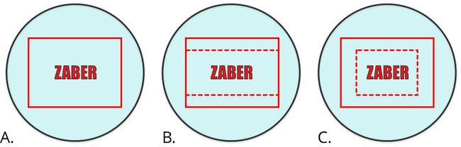
Figure 11. When imaging a specific feature like the Zaber logo here, a single image may be enough. Full coverage of camera (A) captures the logo and a large unnecessary area. Horizontal reduction (B) of the Region of Interest (ROI) increases the maximum frame rate of the camera. Horizontal and vertical reduction (C) of the ROI does not further increase the maximum frame rate of the camera, but it reduces the size of the images output by the camera. This reduces image transfer and processing times yielding improved throughput.
- Pixel binning combines the signal from adjacent pixels into one large virtual pixel. This may help increase sensitivity but will come at the expense of reduced resolution. Binning can improve the speed of acquiring low intensity signals by reducing the duration of exposures. In some cases however, binning can slow the camera down. Some cameras perform vertical binning directly on the CMOS image sensor which does not incur a speed penalty. Horizontal binning is generally performed using the camera’s onboard processor which will reduce the maximum frame rate of the camera. Binning behavior varies from camera to camera. If horizontal binning forces
ISP Enableon, then consider only using vertical binning if maximum speed is required. The resulting compressed aspect ratio may look unusual to a human viewer, but image processing software can compensate for this.
System Settings
Complex multi-channel plate and slide scanning requires precise coordination of X, Y and Z axis positioning, filter cube switching, illumination control, image acquisition, and in many cases image processing. Optimizing the overall system settings can yield large gains in throughput by ensuring all of these steps are carried out in the correct sequence with as few delays as possible.
Latency and Polling
Latency is frequently overlooked as a significant contributor to overall sample scanning time. It may initially appear that shaving a few ms off of serial command transmission is not worth the trouble. However, many small delays can add up to a big impact - particularly when imaging higher density microplates with up to 1536 wells or when executing complex multi-dimensional acquisition sequences. Reducing the windows serial port latency timer to 1 ms is highly recommended.
Reducing the Windows serial latency timer from 16ms to 1ms with the following steps will increase your throughput:
- Ensure you are using a baud rate of 115200 (the default for Zaber ASCII communication).
- Open the Control Panel and Select "Device Manager".
- Under "Ports (COM & LPT)" right click on the COM for use by the device and select "Properties".
- Under the "Port Settings" tab, click "Advanced..."
- Select 1 ms in the drop down menu for the "Latency Timer".
Interrupts
Many system processes are not continuously monitored. Instead, they are polled periodically to check their status. From a computing standpoint, this is efficient, but the delays between when an event occurs, and when the system polls the relevant device or sensor to determine it has occurred can add up quickly on multidimensional imaging of high density microplates.
Interrupts can be used by software to send an immediate notification to the system when an action is complete. Setting the value of comm.alert to “1” (Fig. 12) eliminates the need to wait for the device to be polled, improving process speed and throughput. Enabling comm alerts for move completion eliminates the 8ms polling of serial bus delay for each instruction, which represents 16ms of latency per move.
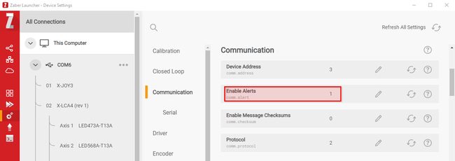
Figure 12. Enabling comm alerts for a device in Zaber Launcher.
Once comm alerts have been enabled, sending positioning commands with the additional waitUntilIdle=False command will significantly improve the throughput by eliminating polling delays. Once set, code will continue to be executed while the stage is moving. To coordinate the movement of multiple axes, each axis will require the axis.waitUntilIdle() to be set.
Microscope Control Software
While the widely used μManager microscopy software supports the coordinated control of a diverse spectrum of hardware from a wide range of manufacturers, this software does have limitations which reduce its maximum sample scanning speed. Its layered architecture introduces delays into the communication with devices. These delays add up quickly with higher density plates with more wells, higher magnification optics require more images per well, and additional excitation wavelengths, Z-stacked focus planes, and time steps.
In addition to communication delays, μManager’s HCS plugin does not generate an optimized scanning path (Fig. 13). The total path length of a μManager scanning pattern for a 96-well plate is 18% further than an optimized “snake” pattern. In addition to taking longer, for continuously operating high-throughput applications, the extra movement distance will result in increased wear on motion stages.

Figure 13. The plate scanning pattern generated by μManager (A) requires 18% more movement than an optimized “snake” pattern (B).
Hardware Triggering
Hardware triggering of cameras by stages, or of stages by cameras can improve imaging throughput by enabling devices to communicate directly with each other. This eliminates the latency penalty of indirect communication via software. Detailed instructions on how to configure triggers are available in the ASCII protocol manual.
Trigger stages with cameras
Hardware triggering can be used to rapidly step though a Z-stack. This is accomplished by setting up a sequence of triggers on the stage that will receive a digital input from the camera and increment the stage position using the /move rel command. When the final position is reached, a position-based trigger on the stage would use the move abs command to return the stage to its initial position.
Moving to arbitrary focus positions is also possible using a stream. The digital output line on the camera should be set to a high voltage level while the exposure is active. The X-LDA focus stage can then be set to detect the exposure active/inactive transition of the camera and step from one position to the next after each exposure has been completed. The basic stream setup where z1 and z2 are arbitrary positions looks like this:
/01 stream 1 setup disable
/stream 1 wait io di 1 == 0
/stream 1 wait io di 1 == 1
/stream 1 line abs z1
/stream 1 wait io di 1 == 0
/stream 1 wait io di 1 == 1
/stream 1 line abs z2
Once setup, the stream can be called with the following commands:
/stream 1 setup live 1
/stream 1 call 1
Many cameras provide both opto-isolated and non-isolated I/O lines. On camera CC01 (Teledyne FLIR BFLY-U3-23S6M-C) the non-isolated line is slightly faster than the opto-isolated line and does not require a pull-up resistor, however without isolation, care must be taken to ensure the voltages stay within the specified nominal range.
Trigger cameras with stages
The digital output line of a Zaber stage can be used to trigger a camera to acquire an image. Communicating directly with a camera eliminates communication delays associated with software triggering. When used with the cloop.settle.tolerance setting on the X-ADR, this can eliminate the need to build an arbitrary setting period into the image acquisition process, increasing throughput. This function is only available for linear motor-driven X-ADR and X-LDA stages. The X-ASR’s motor encoders can detect slips and stalls, but cannot directly measure the vibration and settling of the stages.
Throughput maximization check-list
☐ Securely mount microscope to minimize vibrations and settling time
☐ Optimize motion profile to minimize settling time
☐ Determine minimum required settling time
☐ Enable com alerts
☐ Set Windows COM port latency timer to 1ms
☐ Optimize scanning sequence
☐ Maximum sample-safe illumination
☐ Reduce exposure duration
☐ Maximize camera gain
☐ Turn off onboard image processing by unchecking “ISP Enable”
☐ Disable the “Framerate Enable” setting
☐ Set color cameras to “Raw 8” pixel format
☐ Check camera is running at “Super-Speed” (USB 3.1) and not High-Speed (USB 2.0)
☐ Optimize your Region of Interest (ROI) to minimize excess coverage and overlap