Engineering Multi-Axis Accuracy: A Practical Guide to Precision in Motion Systems
By Graham Kerr, Mechanical Engineering Team
Published on Feb. 18, 2026
Introduction
Many motion control applications require multi-axis movement, ranging from simple XY motion all the way to complex 6 degree of freedom paths. Achieving and maintaining a degree of high accuracy in multi-axis systems is required for everything from ensuring component placement is exact every time to ensuring a sensor has been characterized as you might expect. However, achieving true multi-dimensional accuracy requires special consideration. This article explores the considerations required to attain true multi-dimensional accuracy and equips you with the tools needed to ensure your system is accurate.
Types of Multi-Axis Systems
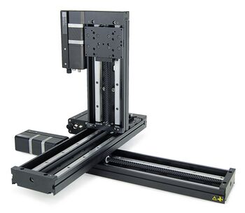
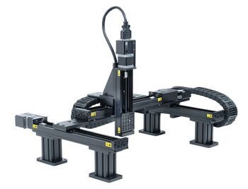
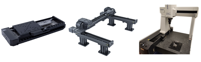
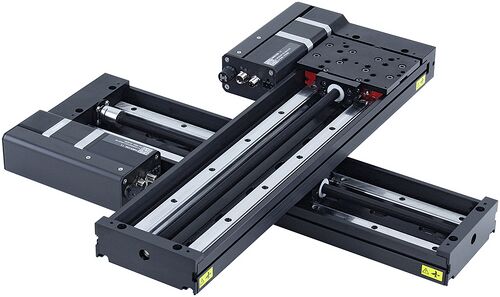
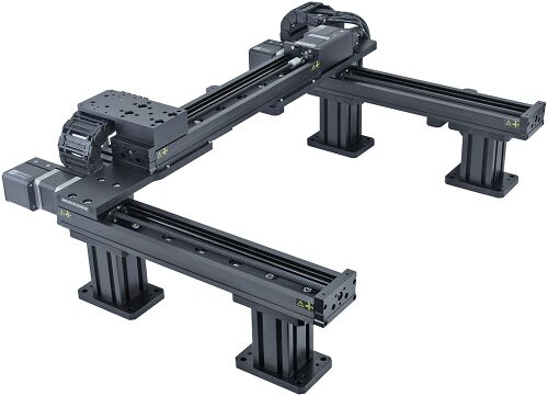
Many different kinds of multi-axis motion systems are used in industry. One of the most common types is known as cartesian systems, which are linear axes combined to form a multi-axis system. These can be split into two main categories: cantilever systems, which consist of singular stacked linear axes, and gantries which have parallel axes to improve load capacity and stiffness.
|
|
|
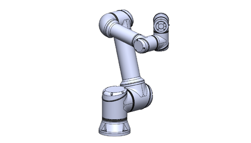
A broad variety of multi-axis systems also exist that are based on rotary axes. The two most ubiquitous types in industry are articulated robot arms and SCARA robots. Articulated robot arms generally have more degrees of freedom, while SCARA arms are faster and more compact.
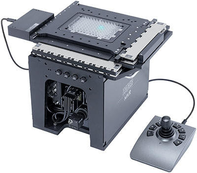
There are also various less-conventional multi-axis motion systems. For example, a microscope like Zaber’s MVR is also a multi-axis motion system; XY axes move the sample horizontally, and a Z-axis is used for focusing. Despite looking quite different, a system like this shares many similarities to cartesian systems.
This article primarily focuses on cartesian systems. As you will learn later, cartesian systems are generally preferred for applications requiring accuracy. However, the concepts presented in the article are generally applicable to all types of motion systems.
The Hidden Complexity of Multi-Axis Accuracy
Linear stages are widely available with excellent accuracy specifications, but it's rare to find accuracy specifications for multi-axis systems. This is true even when the system is made up of a combination of linear stages with well defined accuracy specs. The issue is that system complexity scales rapidly with axis count. While one might assume that two axes have double the complexity of a single axis, the reality is that the complexity scales more like an N2 relationship because angular errors from the first axis compound on the second. This means that a two axis system has more like 4x the complexity of a single axis system!
This is why multi-axis motion systems with true accuracy specifications are surprisingly hard to find. Typical product offerings and their related specifications can be split into three categories:
1. Single axis stages with accuracy specifications:
- These are readily available with excellent accuracy specifications. Even in the case where the multi-axis system is built combining these single axis stages, the overall system accuracy specifications are difficult to calculate.
- Example: Zaber’s linear stages.
2. Multi-axis systems without accuracy specifications:
- Instead of accuracy, manufacturers more commonly list repeatability—a metric that, as we will discuss later, is fundamentally different from accuracy.
- Example: Zaber’s XYZ and gantry systems.
3. Multi-axis systems with accuracy specifications:
- In these cases, the systems are generally expensive or limited to highly specific industries.
- Example: While Coordinate Measuring Machines (CMMs) offer true volumetric accuracy, purchasing and retrofitting such a specialized instrument for a high-precision pick-and-place task is rarely a practical solution.
Why Providing Standard Multi-Accuracy Specs Is Difficult
One reason is that it's difficult to capture meaningful accuracy specifications in a format that can easily be interpreted by a customer. As explained later in the article, there are many different components to multi-axis accuracy, and it’s quite difficult to capture these in a few simple numbers that can be easily understood.
Another reason is that most applications only need certain components of accuracy; for example, XYZ pick and place applications generally only require accuracy in a single XY plane, while imaging applications may only require two dimensional flatness. In general, the multi-dimensional accuracy needs vary widely from application to application. This means that vendors who specify true multi-axis accuracy are inherently producing something that is over-built (and thus overly expensive) for most applications.
Fear not! The saving grace is that many aspects of multi-axis accuracy are highly achievable with a little knowledge. This article gives you the tools to achieve multi-axis accuracy with methods that cost a fraction of buying a specialized system.
Key Takeaways:
- System complexity scales rapidly with axis count.
- Systems with true multi-axis accuracy are hard to find.
- Most applications only need certain components of accuracy.
- Multi-axis accuracy can be readily achieved with a bit of knowledge.
Primer: Fundamentals of Accuracy
Before delving into achieving multi-axis accuracy, there are some fundamental concepts about accuracy that must be understood. These are broadly applicable concepts that can be applied to all types of motion systems.
Accuracy vs Repeatability
Understanding the difference between accuracy and repeatability is critical for working with precision motion systems. This article focuses specifically on accuracy, but these two terms are often misinterpreted and confused. To compare:
- Repeatability: The ability for a motion system to return to the same location over and over.
- If I move to the same position 10 times in a row, how much does the position vary each time?
- Zaber’s definition: The maximum deviation in actual position when repeatedly instructing a device to move to a target position 100 times, approaching from the same direction every time, under stable thermal conditions.
- Accuracy: How close a stage can position to the true requested value.
- If I command the stage to move by 10 mm, how far has the stage actually moved?
- Zaber’s definition: The maximum error possible when moving between any two positions, when both positions are approached from the same direction.
Note that the word precision doesn’t arise here. The word precision is a generic catch-all term with no specific meaning.
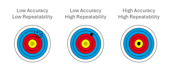
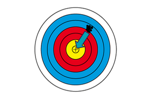
From the image above, an important question arises: which scenario is most indicative of real world systems? Generally, real world motion systems have relatively high repeatability and low accuracy. This characteristic is even more pronounced for multi-axis systems. For example, if you command a robot arm to move to a certain position, it will probably do so repeatedly, but it won’t move to the true position in 3D space you’ve requested.
Thankfully, systems with high repeatability and low accuracy are relatively straightforward to work with. This is because repeatable errors are suitable for calibration; if the error is the same each time, we can apply compensation to remove it.
However, there’s a caveat for the opposite case - if a stage has poor repeatability, calibration will be almost impossible. This means that high repeatability is an important characteristic of stages in a multi-axis system; if you want a certain level of accuracy, it’s important to choose stages with a repeatability higher than the accuracy target. This concept is also applicable to single axis stages, but becomes even more critical for multi-axis applications.
Key Takeaways:
- Accuracy and repeatability are different.
- Most systems have high repeatability and low accuracy.
- High repeatability is important for multi-axis accuracy, because it allows for calibration.
Errors Change Slowly
Another important accuracy related concept is that errors generally change slowly. To summarize this explicitly:
- The derivative of accuracy errors with respect to position is generally low.
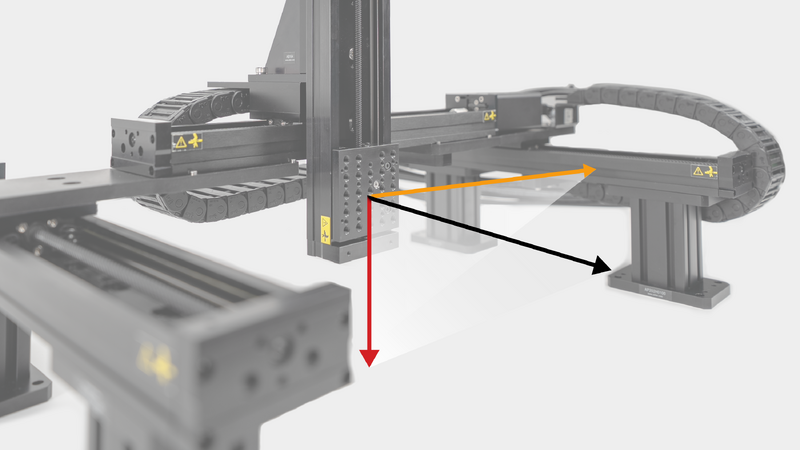
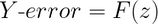
What does this phrase mean? Consider figure 7 below: a common error expected on a gantry system is for the Y-axis to sag due to gravity, causing an accuracy error on the Z-axis. Note that as we move to the left, the Z-axis error changes, but not very quickly. In general, errors that change slowly with position like the one shown below are the norm for most real-world systems.

While this concept may seem evident once it’s been explained, there are major implications; the concept of slowly changing errors is another key factor that makes multi-axis calibration feasible. Because positional errors change gradually, measurement points can be spaced reasonably far apart without sacrificing system accuracy. Contrast this with a hypothetical system where errors change rapidly; such a system would be nearly impossible to calibrate effectively, as the required density of measurement points would be unmanageable. Thankfully, most systems have errors that change slowly with respect to position, working in our favor for calibration.
Key Takeaways:
- Most systems have errors that change slowly with changes in position.
- Slowly changing errors is another key characteristic that allows for calibration.
Case Study - Robot Arms
The concept of errors changing slowly is applicable to most motion systems. However, this isn’t always true, especially for systems with complex kinematics. Robotic arms are one particular case where caution must be exercised.
Compare the gantry system to the robot arm shown below:
- As the gantry moves to the left, its Y-axis stage moves at a 1:1 ratio to the tool-point motion. Because the axis error changes slowly, the tool-point error also changes slowly.
- As the arm moves to the left, the arm passes near a singularity, causing joint J3 to almost entirely invert. Although J3 has an error that changes slowly, it moves so much that the tool-point experiences a large change in error.
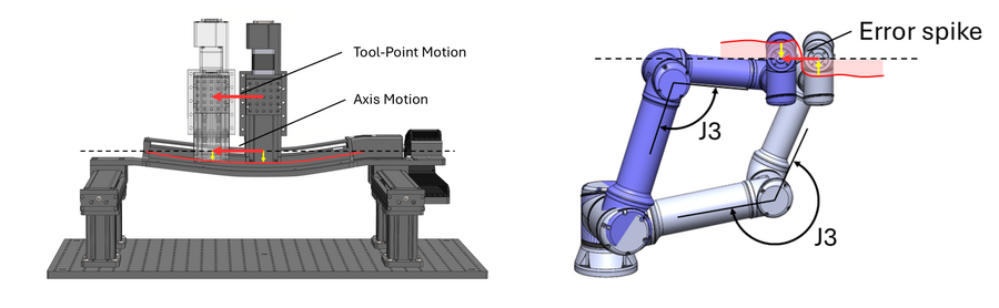
Based on the example above, we’d expect the robot arm to see a sudden change in error whenever it moves near a singularity, which ultimately makes the errors of robot arms difficult to predict. In particular, these rapidly changing errors make robot arms impractical to calibrate, because a high density of calibration points is required at various positions throughout the system travel.
Ultimately, the error mechanisms of robot arms mean that cartesian systems are preferred for applications requiring accuracy.
Abbe Errors
The concept of abbe errors is also of key importance for multi-axis systems. While commonly glossed over for single axis systems, abbe errors are one of the key reasons that make it difficult to create multi-axis accuracy specifications that can be easily captured with a single number.
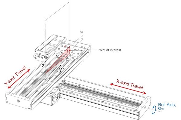
The definition of abbe errors is relatively simple: an angular error, when combined with a linear offset, results in a linear error. For example, consider the XY stage below: angular roll error on the x-axis results in vertical error at the point of interest due to the Y-axis offset.
Abbe errors have various implications for multi-axis systems. First and foremost, it’s important to measure errors at the true point of interest in your system. If calibration points are measured at the stage-top, the errors will be different once an end effector is installed because the offset has changed. To demonstrate a few common examples:
- For a pick and place system, errors should be measured at the center of the gripper jaws.
- For a camera inspection system, errors should be measured at the camera’s focal point.
- For a gluing system, errors should be measured at the glue applicator tip.
Abbe errors also make it important to minimize cantilevering and offsets in multi-axis systems. For example, in an XY system it’s ideal to put the longer travel axis on the bottom so it can be fully supported. Gantries are also ideal for longer travel or higher accuracy systems because the Y-axis is fully supported, removing abbe error contributions from the X-axis stages.
Because gantries are ideal for applications requiring accuracy, the rest of this article highlights examples focused around gantries. However, most of the concepts apply equally to other systems like XY stages.
To learn more about abbe errors, see our article: How Angular Errors (Pitch, Roll, Yaw) Affect Linear Positioning.
Key Takeaways:
- It’s important to measure errors at the tool-point in multi-axis systems.
- Gantries are ideal for applications requiring utmost accuracy, especially at longer travels.
Error Dependency
Understanding the concept of error dependency is also important for multi-axis systems. This concept is straightforward at the high level: for a given error, which axis positions influence it? For example, some errors depend only on the position of a single axis, whereas others depend on the combined position of multiple axes.
To demonstrate error dependency, consider the gantry system below with a misaligned Z-axis. The misalignment creates an error in the Y-direction. However, this error is only dependent on the position of the Z-axis; the error is independent of X and Y axes. In other words:
 |
What this ultimately means is that if we were to calibrate this error - the X and Y positions don’t matter. We could calibrate this error at any XY position, and the error will be eliminated over the full XY travel.

For a more complicated example, consider the flatness error of the X and Y axes. This error depends on both the X and Y positions, but is independent of Z-axis position:
 |
Therefore, in order to calibrate this error, we’d have to measure it over the full X and Y travel range.
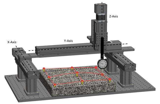
Figure 13: Flatness error depends on the positions of the X and Y axes.
Error dependency ultimately tells us how a given error should be calibrated. Therefore, it’s important to consider these dependencies carefully before calibrating a multi-axis system.
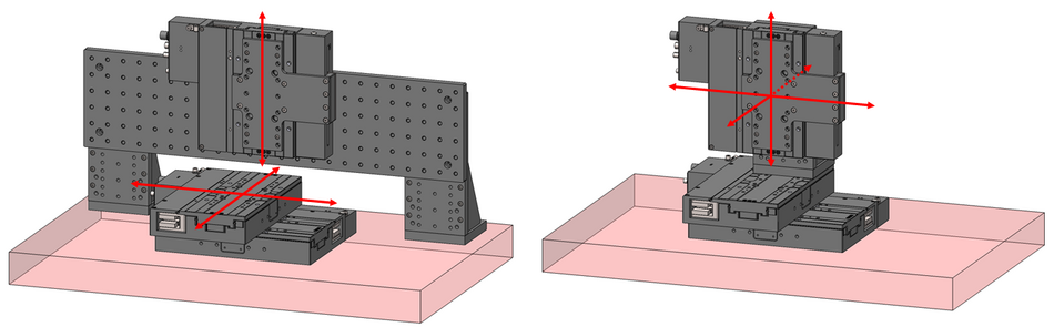
Error dependency can also help with designing the layout of a multi-axis system. For example, a bridge style system can help to isolate Z-axis errors from the X and Y axes because the Z-axis is not stacked on top of the X and Y axes.
Key Takeaways:
- Errors only depend on the position of certain axes.
- Think about dependency carefully when calibrating errors.
Tools for Achieving & Measuring Multi-Axis Accuracy
This article explores various techniques for measuring accuracy errors using high-precision reference artifacts. In most cases, dial indicators paired with granite reference surfaces are highlighted as the standard choice for error measurement, which is due to their wide availability, reasonable cost, and suitable accuracy. However, alternative measuring devices may be substituted depending on the specific accuracy requirements of your system. The following section outlines various equipment that can be useful for measuring multi-axis accuracy errors at a variety of accuracy levels.
The following devices serve as effective alternatives to dial indicators for measuring short distances, particularly when evaluating geometric tolerances such as flatness, parallelism, and perpendicularity against a reference surface. They are presented below in order of increasing precision and cost:
| Measurement Device | Notes |
|---|---|
| Dial indicator (recommended starting point) | This is an excellent starting point for measuring errors down to approximately 5 µm |
| Digital length guage | Length gauges from Mitutoyo or Heidenhain provide higher accuracy, resolution, and can be fully automated. |
| Capacitive sensor | Capacitive sensors can measure nanometer level errors, and are also non-contact. |
These length measurement devices are typically paired with a reference surface to quantify geometric errors. To specifically measure flatness, the table below outlines various reference surfaces that can be utilized in conjunction with a short distance measurement device:
| Reference Surface | Notes |
|---|---|
| Glass | General purpose glass can provide a suitable flatness reference for lower precision systems, especially when sufficiently thick. |
| Aluminum tooling plate | Aluminum tooling plate is another suitable general purpose reference surface, and is typically ground to flatness tolerances of approximately 0.1 mm. Anodizing is useful to prevent wear issues. |
| Granite surface plate
(recommended starting point) | Granite surface plates are the gold standard reference surface. They’re surprisingly cheap and can be obtained with flatness tolerances down to 1 um. Note that granite is less portable than some other options. |
| Optical flat | Glass optical flats can be readily obtained at flatnesses down to 30 nm. These are typically round, but can be custom ordered in various shapes and materials. |
While measuring flatness is relatively straightforward, finding equipment to measure perpendicularity (or squareness) can be more difficult. The table below highlights specialized reference objects designed to be used with short-distance measurement tools to quantify angular errors:
| Reference Object | Notes |
|---|---|
| Machined reference block | A machine-shop fabricated block with perpendicular faces serves as an excellent reference, particularly when validated by a CMM to ensure strict tolerances. While the cost is often comparable to granite equivalents, this approach offers greater flexibility. |
| Machinist's Square | Ground machinist’s squares offer excellent accuracy for compact systems. However, they can be challenging to source in larger sizes and are often impractical for validating systems with extended travel ranges. |
| Granite square
(recommended starting point) | Granite squares are the ideal reference for high precision perpendicularity measurements. They offer superior accuracy while remaining a surprisingly cost-effective solution. |
While the equipment discussed above is ideal for measuring geometric errors like flatness, parallelism, and perpendicularity, measuring linear positioning accuracy is equally critical. This requires instrumentation capable of accurately measuring long distances. The table below presents various options for long-distance measurement, organized from least to most accurate:
| Measurement Device | Notes |
|---|---|
| Digital calipers | For lower precision systems, long-travel digital calipers serve as an accessible option. These devices can typically be sourced in lengths up to 1.5 meters. |
| Linear encoder
(recommended starting point) | Linear encoders are commonly built into linear stages, but can also be purchased standalone in a wide variety of accuracy grades and lengths. A particularly flexible approach involves using a standalone linear scale in conjunction with a magnified camera system to pinpoint reference marks on the scale’s surface. |
| Laser interferometer | Laser interferometers are the gold standard for length measurement. While costly, their potential for accuracy is nearly limitless, constrained primarily by the stability of the testing environment. |
It should be noted that the equipment listed above represents only the most common solutions for measuring multi-axis accuracy errors and is not exhaustive. There are numerous specialized instruments available on the market with varying degrees of accuracy and automation. Furthermore, many of these tools are highly versatile and can be employed for a wide range of metrology tasks beyond the scope of this guide.
How to Correct Common Multi-Axis Accuracy Errors
The following section outlines accuracy errors that are commonly seen in multi-axis motion systems, and provides examples of how to correct them. Note that these errors are demonstrated on gantry systems, but the concepts are applicable to any cartesian motion system.
Misalignment Errors
Misalignment errors, or assembly errors, are errors that occur during assembly of a multi-axis motion system. Ideally, any multi-axis cartesian system should be assembled such that all axes are aligned perfectly orthogonal to each other, and aligned perfectly to the global system reference frame. However, in reality perfect alignment is never possible.
Compared to other error types, misalignment errors are generally the lowest hanging fruit for achieving multi-axis accuracy. This is for two reasons:
- Misalignment errors are usually the largest source of accuracy errors in multi-axis motion systems.
- Misalignment errors are straightforward to correct.
For these reasons, it is generally advisable to correct misalignment errors first, before trying to address other error sources. It’s also important to note that misalignment errors are typically independent of component quality; buying a better stage won’t improve your system accuracy if the stage is installed misaligned.
One other consideration is whether it’s worth addressing misalignment errors in a system being calibrated, or “just letting the calibration handle it”. Generally speaking, it’s worthwhile to mitigate misalignment errors to a practical degree, even if calibration is being employed. Reducing misalignment errors will make the calibration process easier and also make the system less sensitive to things like abbe errors if the system is adjusted after calibration.
Example: X-Axis Parallelism
X-axis parallelism error is a common misalignment error seen on gantry systems. In an ideal system, both of the X-axes should travel perfectly parallel to each other, however in reality the two axes will always be misaligned to some extent.

This type of misalignment typically results in X-axis straightness errors. However, because the Y-axis cannot change length, this error also creates a mechanical overconstraint in the gantry, inducing additional wear and loading on the stages.
To correct X-axis parallelism errors:
- Remove the gantry Y-axis.
- Measure from the carriage of one X-axis stage to the other with a dial indicator.
- Move both stages over the full travel range while monitoring the indicator reading.
- Adjust alignment of the second stage until the indicator reading remains constant.
Note that a dial indicator is the preferred measurement device, but can be substituted for any measurement device of sufficient accuracy for the given application.

One question may arise during correction: how many measurements should be taken along the travel range? In theory, the misalignment should yield a linear error requiring only two measurements to quantify. However, in reality both stages also have straightness errors. For this reason it is recommended to take at least three measurements, or more until the approximate magnitude of straightness error is understood.
You may also note that it’s impossible to fully correct parallelism errors, so what is considered good enough? Generally it is advisable to correct parallelism errors until the total error is approximately on the order of the X-axis straightness errors.
Example: XY Perpendicularity
XY perpendicularity error, or squareness error, is another common error on multi-axis systems. Ideally the X and Y axes should be aligned perfectly perpendicular to each other, but in reality the angle will never be exactly 90°. It should be noted that this type of error is nearly identical to other perpendicularity errors, such as XZ or YZ perpendicularity.

One interesting fact about perpendicularity errors is that they manifest as an error on the opposing axis. For example, when moving the Y-axis stage, the XY perpendicularity error creates a linear error akin to an accuracy error on the X-axis, and vice versa.
Correcting perpendicularity errors is a similar, but slightly more complex process than correcting parallelism errors:
- Place a reference square (typically granite) next to the system.
- Mount a dial indicator to the carriage, measuring on side 1 of the reference square.
- Move the X-axis stages over the full travel range, while adjusting alignment of the reference square until the dial indicator reads constant.
- The square is now aligned to the X-axis.
- Re-mount the dial indicator 90° so it’s facing side 2 of the reference square, ensuring that the reference square alignment is maintained.
- Move the Y-axis stage over the full travel range while monitoring the dial indicator reading to measure the perpendicularity error.
- Adjust the Y-axis alignment until the dial indicator reading is constant.

One important consideration to keep in mind while fixing perpendicularity errors: what is the global reference you want your motion system aligned to? For example, correcting the perpendicularity error above, we’ve assumed that the X-axis is aligned and the Y-axis has an error. However, this could be the exact opposite, and the X-axis might be out of alignment relative to the rest of the system. In most cases, the global system reference will be a feature of importance on the base-plate. The recommended practice is to align the X-axis to the global reference, and then correct squareness errors on the Y-axis.
Gantries also have another important consideration for perpendicularity. The system shown above has a dual drive, where both X-axes are driven by motors using Zaber’s lockstep synchronization feature. Gantries with a passive (unpowered) secondary X-axis are common in industry, but these are not recommended if XY perpendicularity is a concern; the secondary motor will maintain better alignment over the full travel range.
Example: Z Parallelism
A Z parallelism, or vertical parallelism error occurs when the plane of XY motion isn’t parallel to the system’s base. This error results in a height deviation as the motion system moves over the XY travel range.

Note that the example above shows an error on the X-axes, but this error will typically exist on both the X and Y axes.
Z parallelism error is slightly different from the misalignment errors mentioned above. Most misalignment errors can be corrected by loosening off screws and re-aligning the system. However, Z parallelism errors generally exist because of component tolerances and cannot be adjusted as easily. Common methods to correct Z parallelism errors include:
- Shimming parts of the motion system to bring the system parallel to the base.
- Using levelling screws (or jack screws) to bring the system parallel to the base.
With both of these methods, the parallelism error should be measured between the motion system and base-plate using a dial indicator (or similar) while moving over the full XY travel range.
As with other relative errors, it’s important to consider what is the desired global reference plane of your system. For example, the system base-plate is commonly considered the global reference, meaning that parallelism errors should be measured relative to the base. However, in many cases it may be easier to treat the XY motion plane as the true system reference; it could be easier to install a sub-plate with levelling screws and adjust the sub-plate to be parallel with the motion system.

Axis Errors
Axis errors are errors that are intrinsic to each axis of the motion system. The respective errors of each axis combine with misalignment errors to create global system errors. In general, these types of errors are more difficult to work with because they can’t be fixed with alignment, generally requiring calibration to resolve.

Axis errors are directly related to stage quality. For this reason, it is highly recommended to buy quality stages with published precision specifications when designing a motion system where accuracy is a concern. This is especially important because axis errors pose a more complex problem than misalignment errors.
A note to the reader:
With high precision stages like Zaber’s products, axis errors are generally small relative to misalignment errors. This means that axis errors can be safely ignored for many applications. Alternatively, certain applications may have more stringent requirements on specific axes of interest, for example straightness along the X-axis. For cases requiring precision on a specific axis, it is recommended to treat these axes with special attention, either by correcting the specific axis errors with calibration, or using higher precision stages on the axes of interest.
Example: Axis Accuracy
Linear accuracy is one of the most ubiquitous examples of axis errors. The concept of linear accuracy is simple: if we tell a stage to move by a specific distance, the stage won’t have moved that exact distance in reality. The difference between the expected and actual positions is the accuracy error.

Linear accuracy is primarily influenced by a stage’s drive mechanism, which makes component selection a key consideration. When selecting a stage, this is the general ordering of drive mechanisms from least to most accurate:
| Drive Mechanism | Accuracy | Cost | Notes |
|---|---|---|---|
| Belt drive | + | + | Provides longest travel ranges |
| Screw drive | ++ | + | |
| Screw drive with linear encoder | +++ | ++ | |
| Direct drive with linear encoder | ++++ | +++ | Not available for parallel gantries with Zaber controllers |
One useful characteristic about axis accuracy is that error is generally quite linear. This means that the majority of the error can be removed with a simple two-point calibration. While the gold standard for measuring accuracy errors is with a laser interferometer, a two-point calibration can be performed with much more rudimentary equipment. For example, measuring against a machined beam of known length with a dial indicator can provide sufficient accuracy for many applications.

One other note about axis accuracy is that error calibration can be performed before or after assembly into the multi-axis system, depending on which is most convenient. Assembling a stage into the final system generally has minimal impact on the overall accuracy, except in the most stringent cases, where calibration should be performed after assembly.
Example: Axis Straightness
Axis straightness, or straightness of travel, is another common mechanical error seen on linear axes. Straightness error refers to the deviation from the best fit line of travel in the horizontal direction. For example, the travel of a linear axis should be perfectly straight, but in reality this is never the case.
Based on the visualization below, it should be noted that straightness errors cannot be corrected with a simple mechanical adjustment like misalignment errors: they’re intrinsic to the stage. Additionally, straightness errors exist for all axes of the system, despite this image only depicting the Y-axis.

Straightness error is typically measured with a dial indicator and reference straight edge (typically a granite parallel). Because straightness is a deviation from best-fit, the reference edge must be aligned to the theoretical axis of travel. To measure straightness errors:
- Mount a dial indicator on the stage, perpendicular to the axis of interest.
- Position the reference edge to contact the indicator.
- Adjust the reference edge so the indicator reads zero at both opposing ends of travel.
- Move across travel while reading the dial to measure the straightness error.

Once straightness errors are measured, a calibration function must be created in software. One important detail about straightness errors is that they manifest as an error on the opposing axis. For example, a straightness error on the Y-axis creates an error akin to linear accuracy error on the X-axis. Therefore, the calibration function must offset the position of the X-axis, based on the position of the Y-axis:
 |
One other consideration for X and Y axis straightness is that the measurement process is very similar to measuring perpendicularity. If software calibration is already being implemented for straightness, it’s very little work to measure the complete perpendicularity error with a reference square instead of a straight edge, and use the calibration function to correct both perpendicularity and straightness errors.
Example: Vertical Straightness
Vertical straightness, or flatness of travel, is essentially the same concept as axis straightness, but in the vertical direction. Nearly all the concepts from axis straightness apply. However, one key difference is that it is often desirable to measure vertical straightness relative to the machine base, rather than an ideal reference edge, as it may be desirable to capture errors in the machine base.

The calibration function used to correct for vertical straightness errors is also similar to axis straightness. The error is compensated by offsetting the perpendicular axis:
 |
Vertical straightness errors also highlight the benefit of having a Z-axis. For example, if an application requires low vertical errors, it might be desirable to add a Z-axis even if the application only requires XY motion. Adding a Z-axis may also be more cost effective than buying higher precision X and Y axes.
Calibration Methods to Ensure Accuracy
The following section outlines calibration methods that can be used to calibrate many different errors at once in multi-axis systems. This type of calibration focuses less on the individual errors associated with various components of the system, and more so the combination of errors and their resulting global error.
The general process of error calibration is as follows:
- Determine which global system errors are problematic for the application.
- Measure the errors at the point of interest in your system.
- Compensate for the errors as needed with software calibration functions.
The point of interest refers to whatever location is important for the given application, and is generally the tool-point. For more information see this section on abbe errors.

A key detail about error calibration is that it can be as complex as you want. For example, a calibration routine can vary in complexity from compensating for errors in a single direction, to true 3D volumetric error correction. Additionally, more or less calibration points can be used depending on the target system accuracy. For example, the above image shows a 5 x 5 grid of calibration points, but this example could easily be a 3 x 3 grid with minimal loss in accuracy. It is advisable to perform the least complex calibration needed for the given application.
One question that may come to mind: if these methods can compensate for many different errors at once, what is the benefit of the previous sections detailing individual system errors? The answer is that there are many cases where it may only be necessary to compensate for one specific type of error. Additionally, understanding how different errors combine to form global system errors is critical to understanding which errors should be calibrated out, versus correcting with other methods like better system alignment.
Calibration Functions
Another important question may also come to mind: how do I actually go about implementing these calibration functions in software? We recommend referring to our 2D calibration example project, which demonstrates a basic example written in python.
One caveat worth noting is that calibration functions are much easier to apply for point-to-point motions than dynamic trajectories. As such, it is recommended to consider carefully whether your system requires accuracy while it’s moving, or simply at the end-points of motion. For applications requiring dynamic accuracy, the preferred approach is to use Zaber’s PVT feature.
Example: XY Accuracy Calibration
This example demonstrates how to correct global system accuracy errors over the XY travel range. This type of calibration is useful for applications like precision pick and place, where it’s desirable to ensure that a component is placed at the true XY position, or optical inspection, to know the true location of a visual artifact.
The first step is to measure global XY accuracy errors over the system’s full travel range. Shown below is one method to perform this measurement for medium precision applications. A dial indicator mounted at the tool-point measures the location of pockets machined into a precision reference plate. The difference between the expected and measured positions at each point are used to calculate the system errors.

While this method is highly practical for a wide range of applications, similar techniques can be used for different precision levels. For example, higher precision can be achieved using a photolithographic optical target and high magnification vision system. Alternatively, a lower precision approach could be to use a grid printed on a large sheet of plastic and a conventional camera. The approach depends completely on the desired precision level.
One additional consideration is whether the reference features should be directly integrated into the machine. For example, the reference features in the plate shown above could be integrated directly into the sample mounting plate, allowing for easy re-calibration. Alternatively, it could be desirable to have one high-precision master reference if many systems were to be calibrated.
Once error measurement is complete, calibration functions need to be implemented in software. For this calibration, both the X and Y offsets are functions of the errors on both axes:
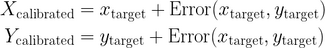 |
Sample code to compute the error function can be found here.
An important caveat for this type of calibration is that it only truly applies at the Z-height where the system errors are measured; when the Z-axis moves to different positions, the error will change to some extent. This means that it’s important to measure system errors at a height as close as possible to the final working plane of the machine. However, the concept of errors changing slowly, tells us that the discrepancy shouldn’t be drastic if the Z-axis position changes slightly, so the calibration will generally provide a satisfactory result for a reasonable distance around the measurement height, especially if misalignment errors on the Z-axis are mitigated.
Example: Z Flatness Calibration
This example demonstrates how to correct global system flatness errors (or Z errors) over the XY travel range. This type of calibration is useful for applications like high precision imaging or microscopy, where vertical deviation would cause the system to lose focus.
A common method of measuring flatness errors is shown below. A dial indicator is mounted at the toolpoint, and measures the errors on a granite surface plate. The system is moved over the full XY travel range while measuring the errors on the indicator.

Figure 30: Measuring flatness errors using a granite surface plate.
One important consideration for this measurement technique is that you may not want the reference surface to be perfect. Like vertical straightness errors, in many cases it is desirable to measure flatness errors relative to the system base, or sample, which will have their own flatness errors. For example, in an imaging application it is generally preferred to calibrate the system flatness relative to whatever surface the sample is mounted on. Measuring relative to a true reference plane is best suited for test and measurement applications.
Once error measurement is complete, calibration functions need to be implemented in software. For this calibration, both the Z offset is a function of the error based on X and Y axis positions:
 |
It should also be noted that this technique can be combined with the previous example, fully eliminating X, Y, and Z errors at one height in the machine. To achieve a true volumetric calibration, these techniques could be repeated at multiple heights, however one plane is likely sufficient for most real-world applications.
Summary
This article outlines many of the key considerations for achieving multi-axis accuracy. Despite seeming highly complex, the nuances of multi-axis accuracy can be readily overcome once the fundamentals and dominant errors are understood. This is especially true given that most applications only require certain aspects of multi-axis accuracy.
In general, the recommended advice is to understand all the concepts presented in this article, and implement the bare minimum required to meet the accuracy requirements of your system. To summarize: fix the errors that matter to you, and don’t go overboard with errors that aren’t important. This approach will provide the most cost effective solution. If you need help deciding which errors matter the most for your task or how to achieve accuracy, please contact our Application Engineering team.