Mastering Motion: Position-Velocity-Time Control for Smooth and Precise Path Planning

Goals

In this article we will show you:

1. how to specify PVT parameters
2. how to validate your trajectories
3. how to command Zaber devices to execute motion along your trajectories

Introduction

Consider the general problem of describing to a computer-controlled machine the specific motion it should produce. A simple approach might be to give the machine a list of coordinates as well as some accompanying action to perform at each coordinate after coming to a stop. This approach is effective when the action a machine performs is only sequentially important, like say dispensing a sample of fluid into an array of containers. But some machine tasks also have critical timing or path requirements — for example, continuously dispensing a line of glue along the perimeter of a tray. In this example, the simple approach above would have difficulty following curved corners and create uneven pools of glue at each stopping point. Similarly, when laser-engraving a logo or text onto a product casing, a naive trajectory might have large speed fluctuations, causing distortion, banding or inconsistent depth in the engraving. Thus it is necessary to use a different approach which defines not only stopping coordinates, but the entire path, with a continuously defined position, which the machine should follow.

Position-Velocity-Time, or PVT, is a flexible algorithm that defines this continuous path in position and time, which we will refer to as a trajectory. PVT trajectories take as an input a list of user-specified control points which act like animation key frames for the motion. The resulting trajectory generated by the PVT algorithm smoothly fills in the path between these control points and is guaranteed to pass through each of these points at exactly the specified position, velocity, and time. These trajectories are capable of describing almost any smooth single or multidimensional path, but choosing the correct parameters can be difficult and sometimes unintuitive.

Many Zaber devices are capable of accepting PVT sequence data (the user-specified control points mentioned above) and executing moves based on calculated PVT trajectories. The trajectory calculation happens in device firmware. User-specified PVT sequence data can be loaded onto a device by several different means including using our Zaber Launcher application, using your own code with our Zaber Motion Library API, or by direct serial communication with devices using our ASCII communication protocol.

It can be a challenging first step in this process to determine complete and well-formed PVT sequence data to send to your devices. To make this step easier we have created some helper classes which can be found in the the following Git repository:

 zaber_examples/examples/motion_pvt_sequence_generation

This article demonstrates how to use these helper classes to generate complete PVT sequence data, how to use the PVT Viewer feature of Zaber Launcher to visualize the corresponding trajectory, thus validating the PVT sequence data, and finally how to use the PVT Viewer to load the PVT sequence data onto connected Zaber devices and have those devices execute moves according to the calculated PVT trajectory.

Specify the parameters

Time (s) Axis 1 Position (cm) Axis 2 Position (cm) Axis 1 Velocity (cm/s) Axis 2 Velocity (cm/s) 0 0 2 0 0 2 2 0 1 -1 4 2 1 -1 1 5 1 0 0 0 Table 1: An example set of PVT control points.

Figure 2: An example PVT trajectory generated from the set of control points.

The faded dashed line shows the path of the sequence from start to end, and the faded points and arrows make up the control point positions and velocities. The velocities are shown as vectors combining the x and y components. It's easy to see that the motion is smooth, and we can create a fairly complex movement with only a handful of points.

It's also useful to define a few concepts that are illustrated in Figure 2.

1. A PVT point is a control point that defines the position and velocity of one or more axes at a specific moment in time. There are 4 PVT points in Figure 2.
2. A PVT segment is the trajectory between two PVT points. It defines the position, velocity, and all other trajectorial information at any time between its two composing points. It only depends on its two composing points. There are 3 segments in Figure 2, or one for each point-pair.
3. A PVT sequence is the trajectory through a collection of PVT points. Because each segment only depends on its two composing points, the sequence essentially stitches together all the segments formed from each point pair. This is represented by the entire trajectory in Figure 2.

In the above example, we started with a fully-defined PVT sequence. Often-times, however, some parameters are definitively known and others need to be inferred or calculated. One example might be a multi-axis sequence where we want to pass smoothly through a set of known position control points but don't necessarily know or care about the velocity or time through which to pass them. Another example might be a single-axis sequence where we have position-time data and want to generate a trajectory that passes through each point with some sensical velocity which we don’t strictly define except that it shouldn’t cause problems. In these cases, we can generate missing parameters using code from our PVT Sequence Generation example repository. We'll also see that often sequences that make use of these generated parameters have some advantages over manually specified ones.

When velocity is unknown

If position and time are already known at all points in the sequence, we can calculate the missing velocity values by specifying some other useful property of the underlying motion paths. One common way of doing this is to enforce that acceleration has no sudden jumps anywhere in the sequence. Though we will not go into the math in this article, you can find an implementation of the algorithm in the accompanying repository. Forgoing these details, you can generate the missing velocities for a position-time sequence with a couple simple lines of python code, using the helper classes in the pvt.py file of the accompanying repository:

# Import the helper classes
import pvt
# Define the sequence of time values, in seconds.
time_sequence = [0, 2, 4, 5]
# Define the sequence of position values, in centimetres. Note
# we use a 2-D array for the position sequence.
position_sequence = [
    [0, 2, 2, 1],  # axis 1 positions
    [2, 0, 1, 0]   # axis 2 positions
]
# Create a sequence, generating the missing velocity values
pvt_sequence = pvt.Sequence.generate_velocities(time_sequence, position_sequence),
# Save the sequence to a file for import to the PVT Viewer App
pvt_sequence.save_to_file("my_sequence_generated_velocities.csv")

The above code saves the fully-specified sequence to a CSV file compatible with our PVT Viewer App in Zaber Launcher. The Validate the sequence section of this article describes how you can import this sequence in the app to visualize and validate the position, velocity, and acceleration trajectories. The Execute motion along the calculated trajectory section of this article describes how to command a connected device to follow the trajectory.

The resulting motion is shown below. This time, the acceleration vector is shown with the green arrow.

Note that the green arrow doesn't suddenly jump at the control points, and the resulting motion looks very smooth. Compare this to the case where we specify the velocities manually. We can very clearly see sudden jumps in the acceleration vector each time the sequence reaches one of the control points.

We can see the difference between the generated and specified cases even more clearly by plotting the position, velocity, and acceleration profiles over time, as shown in the following figure for axis 1.

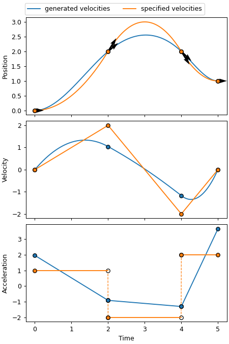
Some takeaways:

1. There are never sudden jumps in position or velocity, regardless of how the parameters are specified. This is true for any PVT-generated trajectory.
2. The position trajectories pass continuously and smoothly through each of the generated points.
3. The velocity trajectories pass through each of the points, but the trajectory with generated velocities is smoother.
4. There are no sudden acceleration jumps in the generated-velocities case.

Besides the obvious effects on motion smoothness, sudden jumps in acceleration can have some negative effects on the system. For example, they can lead to accelerated mechanical wear, position overshoot in flexible systems, and backlash effects in screw-based drive systems. On the other hand, sometimes it is preferable to be able to specify velocity manually. For example, if we are close to a travel range limit and need to shape the curve in such a way as to not break it, or if we want to control the speed of the path at the control point.

When position is unknown

Similar to the previous section, we can generate missing position values by calculating them from the constraint that acceleration is continuous. Unlike the velocity case, however, we also have to impose one additional constraint, which is that starting acceleration is zero. Using the helper classes in the pvt.py file of the accompanying repository, you can generate the missing positions for a velocity-time sequence in CSV form with a couple simple lines of python code.

import pvt
# Define the sequence of time values, in seconds.
time_sequence = [0, 1, 2, 3, 4]
# Define the sequence of velocity values, in centimetres per second.
velocity_sequence = [
    [0, -4, 0, 16, 0],   # Axis 1 velocities
    [-2, 0, 8, 0, 0]   # Axis 2 velocities
]
# Create a sequence, generating the missing position values
pvt_sequence = pvt.Sequence.generate_positions(time_sequence, velocity_sequence)
# Save the sequence to a file
pvt_sequence.save_to_file("my_sequence_generated_positions.csv")

The resulting motion is shown below.

Note that the resulting motion is smooth and the path passes through each of the generated positions with the specified velocities. Also note that the start acceleration for the sequence is zero. This is a constraint enforced by this generation function, and will always be the case when generating positions from it.

When velocity & time are unknown

The previous two sections assumed the time parameters were known. For multi-axis systems, the time parameter is the most difficult to specify, as it directly couples the axes together. For example, in a two-axis system, reducing the time of one point may improve the smoothness of one of the axis trajectories, but make the other worse.

Once again, we can generate the missing parameters using one of the helper classes in the pvt.py file of the accompanying repository. You'll note that, unlike the previous cases, we need to define a target speed and acceleration for the generation algorithm. The algorithm uses these values to find suitable velocities and times for the given position changes. A higher target acceleration will result in shorter times between points when moving slower than the target speed, and a higher target speed will result in shorter times between points when traveling near the target speed. It's important to understand that these targets don't specify limits, they simply provide a reference.

You'll also notice we specify a resample number. This means we're telling the generation algorithm to generate a path and then instead of using the exact control points we requested, split the path up into some number of equal-length segments. The resulting path will still travel through or very close to the specified position values. While it's not necessary to specify a resample number, it is recommended as it produces smoother motion.

import pvt
# Set a target speed and acceleration.
target_speed = 20  # cm/s
target_accel = 100  # cm/s²
position_sequence = [
    [0, -4, 0, 16, 0],
    [-2, 0, 8, 0, -32],
]
# Specify a number of points to resample the generated path by
resample_number = 10
# Create a sequence, generating the missing parameter values
pvt_sequence = pvt.Sequence.generate_times_and_velocities(position_sequence, target_speed, target_accel, resample_number)
# Save the sequence to a file
pvt_sequence.save_to_file("my_sequence_generated_velocities_and_times.csv")

The resulting motion is shown below.

As you can see, the 5-point path has been resampled into 10 points with equal segment lengths, and the resulting motion is smooth in both position and velocity. You can use an even higher resample number to smooth out the velocity even more. Let's look a bit closer at the trajectories.

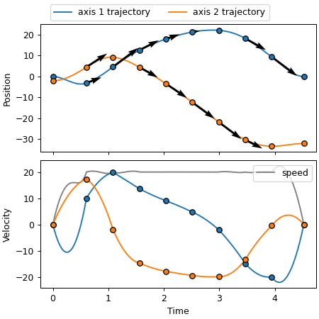
You'll notice the speed, which is the vector sum of the axis 1 and axis 2 velocities, approximates a trapezoidal shape. This shape is a result of how the generation algorithm works. Essentially, it creates a purely spatial path through the specified position points, and then calculates the velocity and time parameters by following this path using a trapezoidal motion profile.

Note that you can elect not to resample the path and use the given control points by not specifying a resample number.

...
# Create a sequence, generating the missing parameter values without specifying a resample number
pvt_sequence = pvt.Sequence.generate_times_and_velocities(position_sequence, target_speed, target_accel)
...

The resulting path is still smooth, but has some speed oscillations which may be undesired.

Validate the sequence

Once we have created a fully-specified PVT sequence, we may find problems with it when trying to send it to a device and command the device to calculate and follow the corresponding trajectory. Usually, this is due to trajectories falling outside position or velocity limits. When sending PVT commands to a Zaber device via Zaber Motion Library or the ASCII protocol, the device will automatically reject points that would break such a limit. To understand why a point is failing, however, or to validate the shape of the resulting trajectory, it's often best to visualize it. This can be done with the PVT Viewer App in Zaber Launcher.

The accompanying repository contains a number of sample CSV files you can use for importing. For example, try importing the file wave_1d.csv. The app will load the sequence, but immediately recognize a problem. The start and end velocities are nonzero. To fix this, we simply need to open the file in a text editor and set the start and end velocities to zero. Once the modified file is saved, the PVT Viewer App will automatically incorporate the changes.

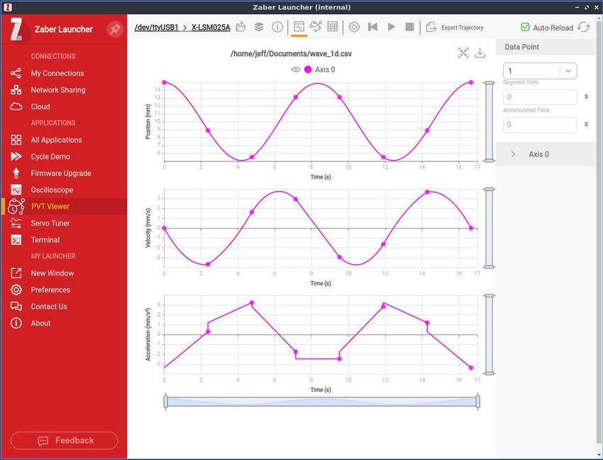
In the app, we can also connect a device to validate the positions and velocities of the sequence against the device's position and speed limits. These limits will be displayed directly on the plots, making it easy to identify what part of the sequence is problematic.

General debugging tips

Before jumping into the more advanced debugging techniques, consider these more high-level tips:

1. When sending PVT points directly to a Zaber device, be mindful of the following distinctions compared to how PVT has been presented in this article. For more information, see the PVT section of the ASCII protocol manual.
   • Times are specified as relative times or durations since the previous point.
   • The starting point (time=0) is inferred from the current state of the device.
   • Positions can be specified absolutely or relatively.
2. Ensure that the velocity at the start and end of the sequence is zero.
3. Avoid specifying position or velocity values that are very close to device limits. PVT sequences become increasingly difficult to debug as this happens, as trajectories are more likely to briefly exceed axis limits when control points are close to them.

Identify problematic points

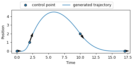
Recall that the trajectory through a particular segment is fully defined by its two composing points. What that means is that to address an issue occurring somewhere in a PVT sequence, we can modify either or both of the two points that make up the segment in which the issue occurs. For example, in Figure 11, the second and third control points have positions 1 and 2, respectively. The segment that they create, however, peaks past position 4, far outside their bounds. In some systems, this could cause the axis to exceed its travel range. Plainly, the generated trajectory would crash into the physical end of the device. To reduce the magnitude of this peak, we would look at its two enclosing points, or points 2 and 3 in the sequence.

Reduce large position peaks

Some point-pairs may generate large position peaks. If the peak exceeds the travel range of the device, for example, it would cause the stage to hit one of its limits. Usually, a large position peak is caused by too large a velocity over too large a period of time. Address this either by:

1. Reducing the duration of the problem segment:
   

   

   Figure 12: Reducing the time of a segment with large position peak.
2. Reducing the velocity magnitudes of the problem segment's composing points:
   

   

   Figure 13: Reducing the speed of a segment with large position peak.
3. Adding an intermediate zero-velocity point:

   

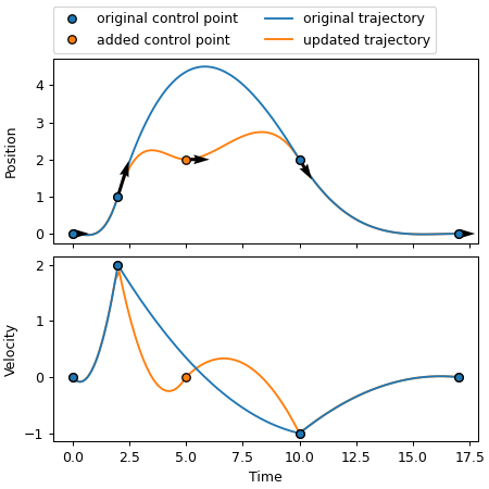
   Figure 14: Adding a zero-velocity point to a sequence with large position peak.

Reduce large velocity peaks

Some point-pairs may generate trajectories with large velocity peaks. If the peak exceeds the speed limit of the device, it could cause the motion to fail or the device to stall. Usually, a large velocity peak is caused by too big a position change over too small a time. Address this by:

1. Increasing the duration of the problem segment:
   

   

   Figure 15: Increasing the duration of a segment with large velocity peak.
2. Reducing the position change of the problem segment:
   

   

   Figure 16: Reducing the position change of a segment with large velocity peak.
3. Increasing the velocity magnitudes of the problem segment's composing points:
   

   

   Figure 17: Increasing the speed of a segment with large velocity peak.

Execute motion along the calculated trajectory

Once we've reshaped the trajectory to our liking, we can send the PVT sequence to a connected device and command the device to calculate and follow the corresponding trajectory directly from the PVT Viewer App by hitting the play button. The app will track the live position, velocity, and acceleration of the device as it follows the path.

Closing thoughts

PVT is a powerful and flexible algorithm because it can define nearly any motion you can imagine across as many axes as you wish. For example, it can define the trajectory of a single linear actuator or the coordinated movements of a 6-axis robot arm.

While flexible, PVT-generated trajectories can behave in unintuitive ways between the specified control points because the trajectory through these regions is sensitive to the chosen parameters. In applications where only certain parameters are known — for example when wanting a set of connected axes to trace out a specific shape without any specific requirement for velocity, or when wanting one or more axes to be at specific positions at specific times — choosing or generating the right values for the remaining parameters is not always obvious. This is especially true when dealing with multi-axis systems, where parameters for each axis must be chosen with consideration to all other axes. Once all parameters are specified, we need a way to validate the generated trajectory for the system we wish to follow it on and, if necessary, fix any problematic segments by making small changes to the parameters.

With the workflows presented in this article and the helper classes in the accompanying git repository, you can specify complete PVT sequences, generating any missing parameters as necessary. Use the PVT Viewer App in Zaber Launcher to visually validate the resulting trajectory. Send the PVT sequence to a connected Zaber device and command the device to calculate and follow the corresponding trajectory either directly in Zaber Launcher, using Zaber Motion Library, or through the ASCII protocol.

Appendix: PVT equations

Although PVT represents a generic class of algorithms, one of the most common, and the one that Zaber uses internally, is a cubic polynomial fit. The position over each segment is generated from a cubic polynomial function of time, where the coefficients are calculated using the positions and velocities at the start and end of that segment. A multi-axis sequence works the same way, with distinct polynomials for each segment on each axis.

The cubic equations can be expressed in continuous or discrete time. At larger time scales, the two sets of equations produce nearly-identical trajectories. However, at small time scales, the results may slightly differ. Generally speaking, we recommend using the continuous representation in most cases as it is simpler, uses standard units, and does not depend on a particular sample time.

Continuous representation

The continuous equations describing the position p and velocity v at any time t in a particular segment are:

(1)

where,

• c₀, c₁, c₂, and c₃ are the polynomial coefficients

The polynomial coefficients are calculated by solving the set of equations formed by the start and end conditions:

(2)

where,

• pᵢ and p₂ are the positions at the start and end point
• v₁ and v₂ are the velocities at the start and end point
• t₁ and t₂ are the times at the start and end point

Note that position, velocity, and time must be expressed in similar units. E.g., if position is in centimetres and time is in seconds, velocity must be expressed in centimetres per second.

Discrete representation

The discrete equations describing the position p and velocity v at any sample index T in a particular segment are:

(3)

where, again,

• c₀, c₁, c₂, and c₃ are the polynomial coefficients
• v[T] is the discrete velocity at sample index T, equivalent to p[T] - p[T - 1]

The coefficients can be calculated in the same way described as for the continuous case, by solving the set of equations formed by the start and end conditions.

Note that position, velocity must be expressed in similar units relative to the real-world time between sample indices. E.g., if position is in centimetres, velocity must be expressed in centimetres per sample period.